This question has bothered me occasionally over the years and I’ve never really come to what I felt was a satisfactory answer. The choice of a loss function is really a choice about the assumed noise distribution. A mean squared error loss function, for example, corresponds to an assumption that the noise in the system to be modeled is Gaussian. Noise in the firing rate of neurons is often assumed to follow a Poisson distribution.
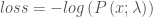
In the Bayesian framework, the noise distribution is also known as the likelihood. Converting a likelihood to a loss function is just a matter of taking the negative log of the the likelihood distribution:
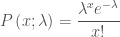
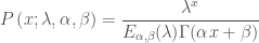
Writing this in terms of the measured firing rate, 


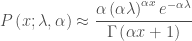
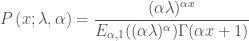
The use of the Poisson distribution as a noise model carries with it the assumption that within a given time window, the variance of the firing rate is equal to the mean of the firing rate. The parameter that determines the mean and variance in the Poisson distribution is 
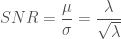
This all makes sense, we would want and expect higher firing rates of neurons to have higher SNR, otherwise it would be hard to transmit information and would be a tremendous waste of energy. But the relevant questions are:
1) Is the mean and variance of the firing rates of real neurons coupled as predicted by the Poisson distribution?
2) And if not, what are the consequences of the difference and how can we fix it?
The answer to the first question is a definite NO. For neurons driven by natural stimuli, their responses are clearly sub-Poisson; the variance of the firing rate is lower than the mean of the firing rate. For example, here are plots of the mean vs the variance of firing rates in each of 2000 16.6ms bins for two neurons in V1. The mean and variance seem to be linearly related, but the slope is clearly less than 1. The slope in each plot is essentially the Fano Factor for each neuron. The parameter 


So, higher firing rates have even higher SNR than predicted by the Poisson distribution. This is good for energy use in the brain, but seems to be bad for the standard Poisson loss function. The Poisson loss function may not give enough credence to the SNR of high firing rates. Models fit with the Poisson loss function could thus be more influenced by lower firing rate time bins and less influenced by higher firing rate time bins than one would want, given that the noise is actually sub-Poisson.
So how can we fix this? Can we modify the Poisson distribution with an extra parameter,


After playing with the equation for the Poisson distribution for a while, I worked out this approximate distribution function:
This function isn’t an exact distribution function, it doesn’t sum to exactly 1 for every setting of 


This is nice, but it seemed a bit contrived to me. While trying to find some connection to the literature, I came across this paper which generalizes the Poisson distribution using the Mittag-Leffler function:
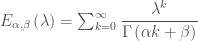
The Mittag-Leffler function generalizes the exponential function; the exponential corresponds to setting 
The formulation, however, breaks the connection between 


This exact distribution relates to the approximate distribution function presented earlier, because as it turns out, the Mittag-Leffler function can in this case be well approximated as:

Making this substitution returns the approximate distribution function above. Now that this approximation has a little more mathematical grounding, we can return to the question of appropriate loss functions for neurons. For reference, let’s first plot the squared error loss function. We see that this loss function is minimized when a model’s prediction 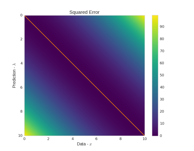
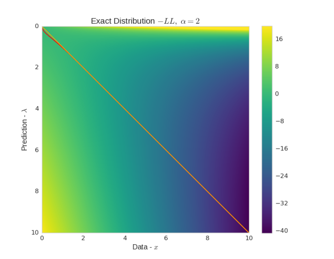
We can turn both the exact distribution function and the approximate distribution function described above into loss functions by taking their negative log. Let’s now plot the exact distribution function’s negative log likelihood when 
 Now let’s plot the approximate distribution function’s negative log likelihood when
 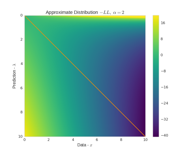 This loss function is nearly identical, but is unbiased. It’s also much easier to deal with since there’s no infinite summation. However, after dropping constants, scaling factors and terms that don’t depend on the model parameters, we get:
which is just the standard Poisson loss function!
This was surprising to me at first, so I investigated a related model that has a similar linear coupling between the mean and variance, the quasi-Poisson model. (The quasi-Poisson model also has a corresponding approximate distribution function that I found is actually less accurate is most situations than the one proposed here, but that’s really not worth getting into as we’ll see). The mean and variance in the quasi-Poison model are defined as:


And a quasi-Poison GLM is defined as:

with 


![\hat {\beta }^{\left[ j+1\right] }=\left( X'W^{\left[ j\right] }X\right)^{-1}X'W^{\left[ j\right] }\overline {y}^{\left[ j\right] }](https://s0.wp.com/latex.php?latex=%5Chat+%7B%5Cbeta+%7D%5E%7B%5Cleft%5B+j%2B1%5Cright%5D+%7D%3D%5Cleft%28+X%27W%5E%7B%5Cleft%5B+j%5Cright%5D+%7DX%5Cright%29%5E%7B-1%7DX%27W%5E%7B%5Cleft%5B+j%5Cright%5D+%7D%5Coverline+%7By%7D%5E%7B%5Cleft%5B+j%5Cright%5D+%7D&bg=ffffff&fg=444444&s=0&c=20201002)
and the weighting function:

However, notice that when you substitute 

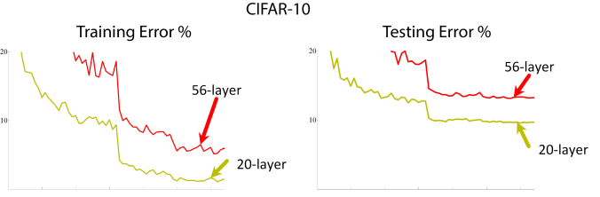 It would seem that for standard architectures and training methods, we’ve passed the point of diminishing returns and started to regress. The theoretical benefits of increased depth, will never be realized unless we do something differently. We must go deeper!
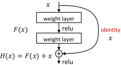
 The residual learning blocks can thus be thought of as implementing
You must be logged in to post a comment.